The is a data package with an excerpt from the Gapminder data. The main
object in this package is the gapminder data frame or
“tibble”. There are other goodies, such as the data in tab delimited
form, a larger unfiltered dataset, premade color schemes for the
countries and continents, and ISO 3166-1 country codes.
The gapminder and gapminder_unfiltered data
frames include six variables, (Gapminder.org
documentation page):
| variable | meaning |
|---|---|
| country | |
| continent | |
| year | |
| lifeExp | life expectancy at birth |
| pop | total population |
| gdpPercap | per-capita GDP |
Per-capita GDP (Gross domestic product) is given in units of international dollars, “a hypothetical unit of currency that has the same purchasing power parity that the U.S. dollar had in the United States at a given point in time” – 2005, in this case.
The package contains two main data frames or tibbles:
-
gapminder: 12 rows for each country (1952, 1957, …, 2007). It’s a subset of … -
gapminder_unfiltered: more lightly filtered and therefore about twice as many rows.
Note: this package exists for the purpose of teaching and making code examples. It is an excerpt of data found in specific spreadsheets on Gapminder.org circa 2010. It is not a definitive source of socioeconomic data and I don’t update it. Use other data sources if it’s important to have the current best estimate of these statistics.
Install and test drive
Install gapminder from CRAN:
install.packages("gapminder")Load it and test drive with some data aggregation and plotting:
library(gapminder)
library(dplyr)
library(ggplot2)

aggregate(lifeExp ~ continent, gapminder, median)
#>   continent lifeExp
#> 1    Africa 47.7920
#> 2  Americas 67.0480
#> 3      Asia 61.7915
#> 4    Europe 72.2410
#> 5   Oceania 73.6650

gapminder %>%
  filter(year == 2007) %>%
  group_by(continent) %>%
  summarise(lifeExp = median(lifeExp))
#> # A tibble: 5 × 2
#>   continent lifeExp
#>   <fct>       <dbl>
#> 1 Africa       52.9
#> 2 Americas     72.9
#> 3 Asia         72.4
#> 4 Europe       78.6
#> 5 Oceania      80.7

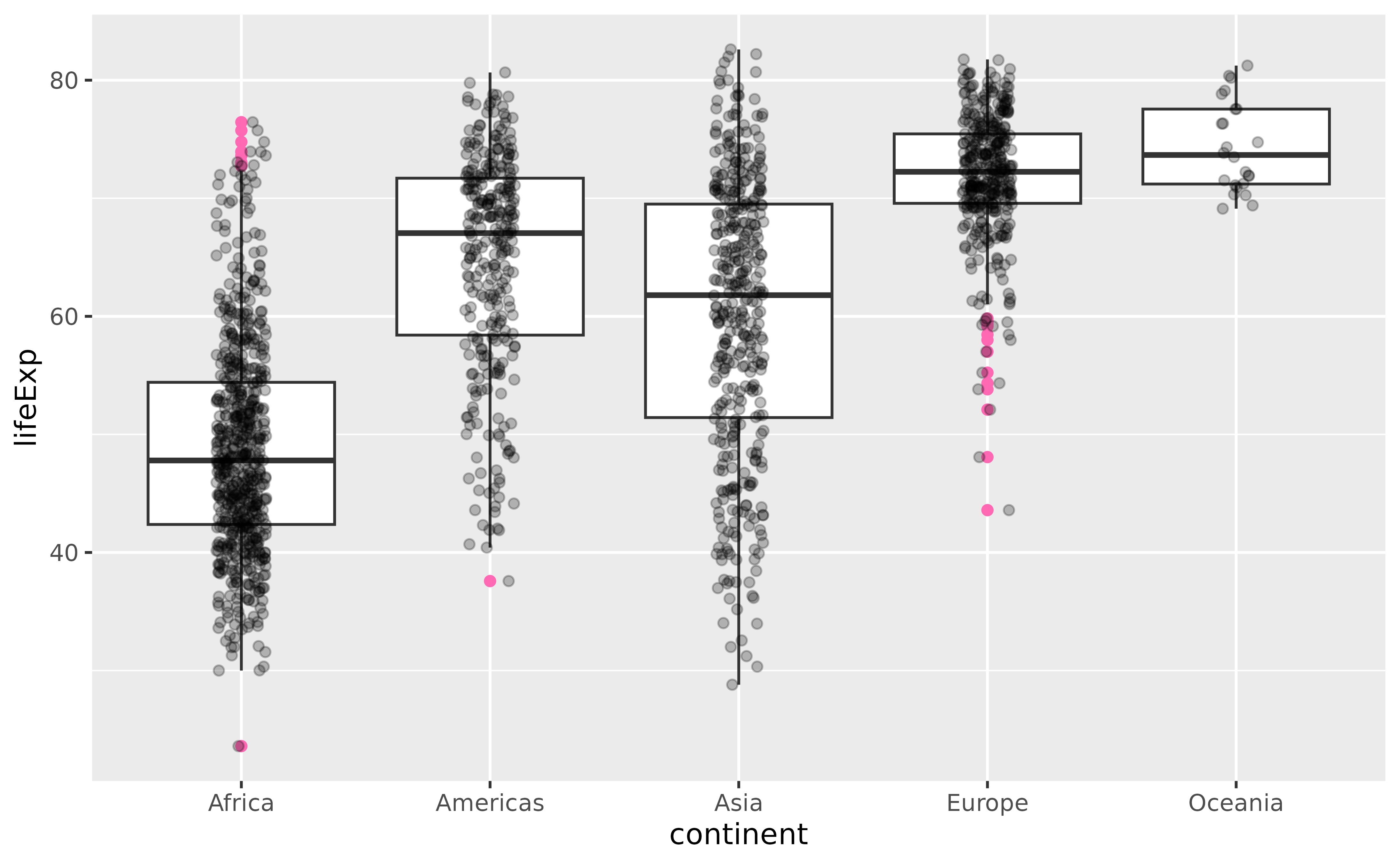
ggplot(gapminder, aes(x = continent, y = lifeExp)) +
  geom_boxplot(outlier.colour = "hotpink") +
  geom_jitter(position = position_jitter(width = 0.1, height = 0), alpha = 1 / 4)
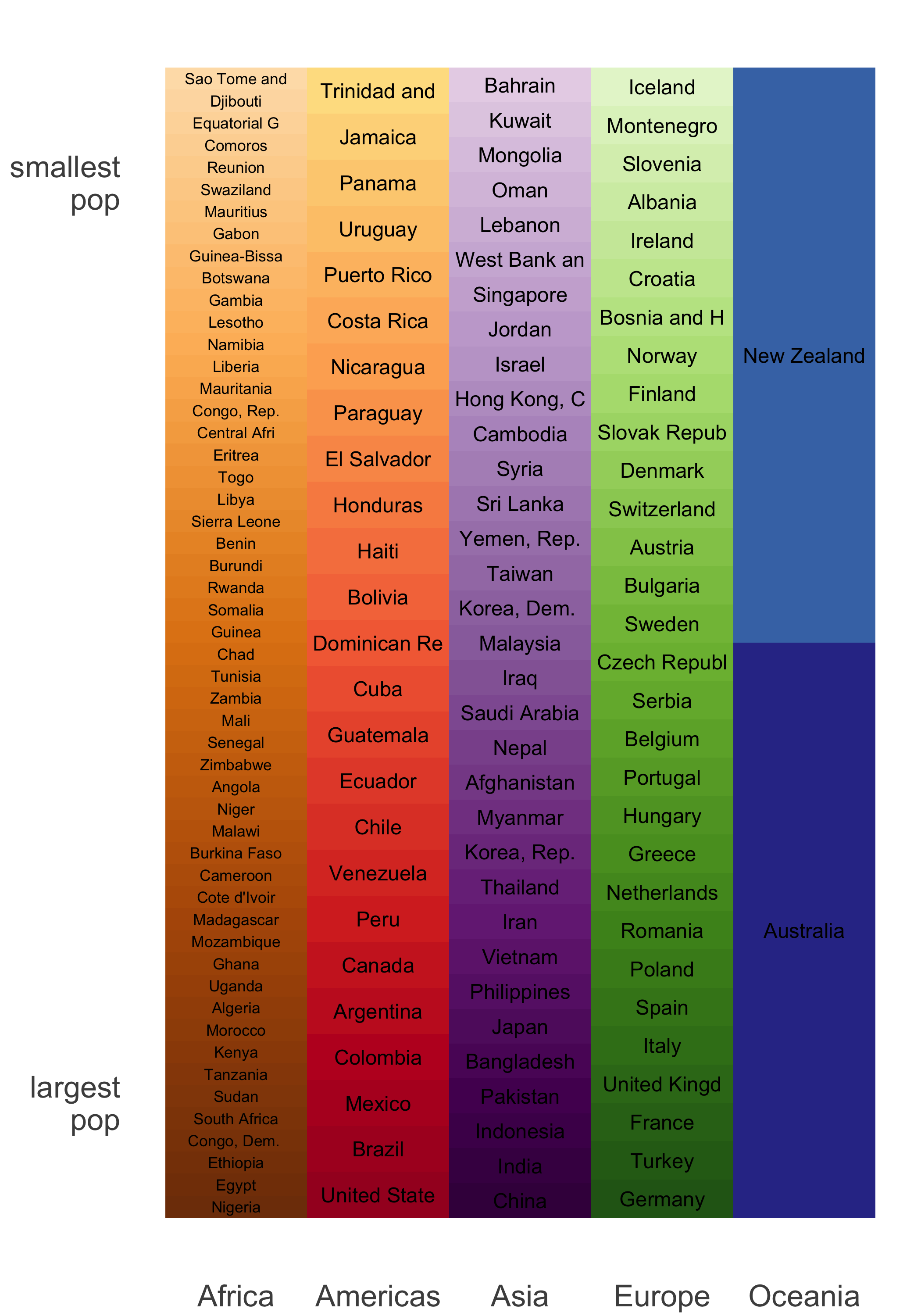
Color schemes for countries and continents
country_colors and continent_colors are
provided as character vectors where elements are hex colors and the
names are countries or continents.
head(country_colors, 4)
#>          Nigeria            Egypt         Ethiopia Congo, Dem. Rep.
#>        "#7F3B08"        "#833D07"        "#873F07"        "#8B4107"
head(continent_colors)
#>    Africa  Americas      Asia    Europe   Oceania
#> "#7F3B08" "#A50026" "#40004B" "#276419" "#313695"
The color schemes are available as:
- PNG or PDF, in the package’s GitHub repo
-
continent-colors.tsvandcountry-colors.tsv, which are part of the installed package
How to use the color scheme in ggplot2
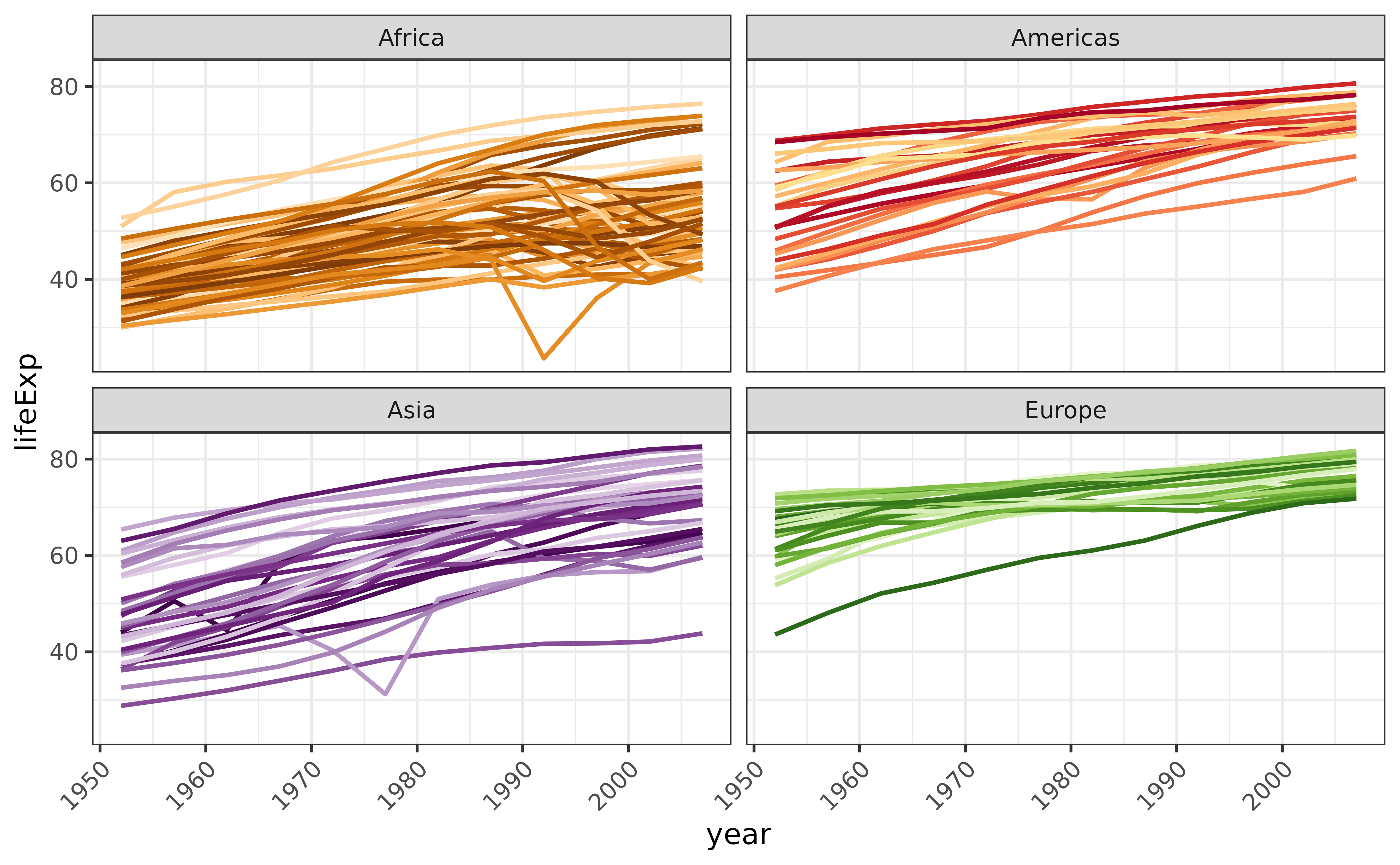
Provide country_colors to
scale_color_manual() like so:
... + scale_color_manual(values = country_colors) + ...
library("ggplot2")

ggplot(
  subset(gapminder, continent != "Oceania"),
  aes(x = year, y = lifeExp, group = country, color = country)
) +
  geom_line(linewidth = 0.8, show.legend = FALSE) +
  facet_wrap(~continent) +
  scale_color_manual(values = country_colors) +
  theme_bw() +
  theme(
    strip.text = element_text(size = rel(0.8)),
    axis.text.x = element_text(angle = 45, hjust=1)
  )
How to use the color scheme in base graphics
# for convenience, integrate the country colors into the data.frame
gap_with_colors <-data.frame(
  gapminder,
  cc = I(country_colors[match(gapminder$country, names(country_colors))])
)

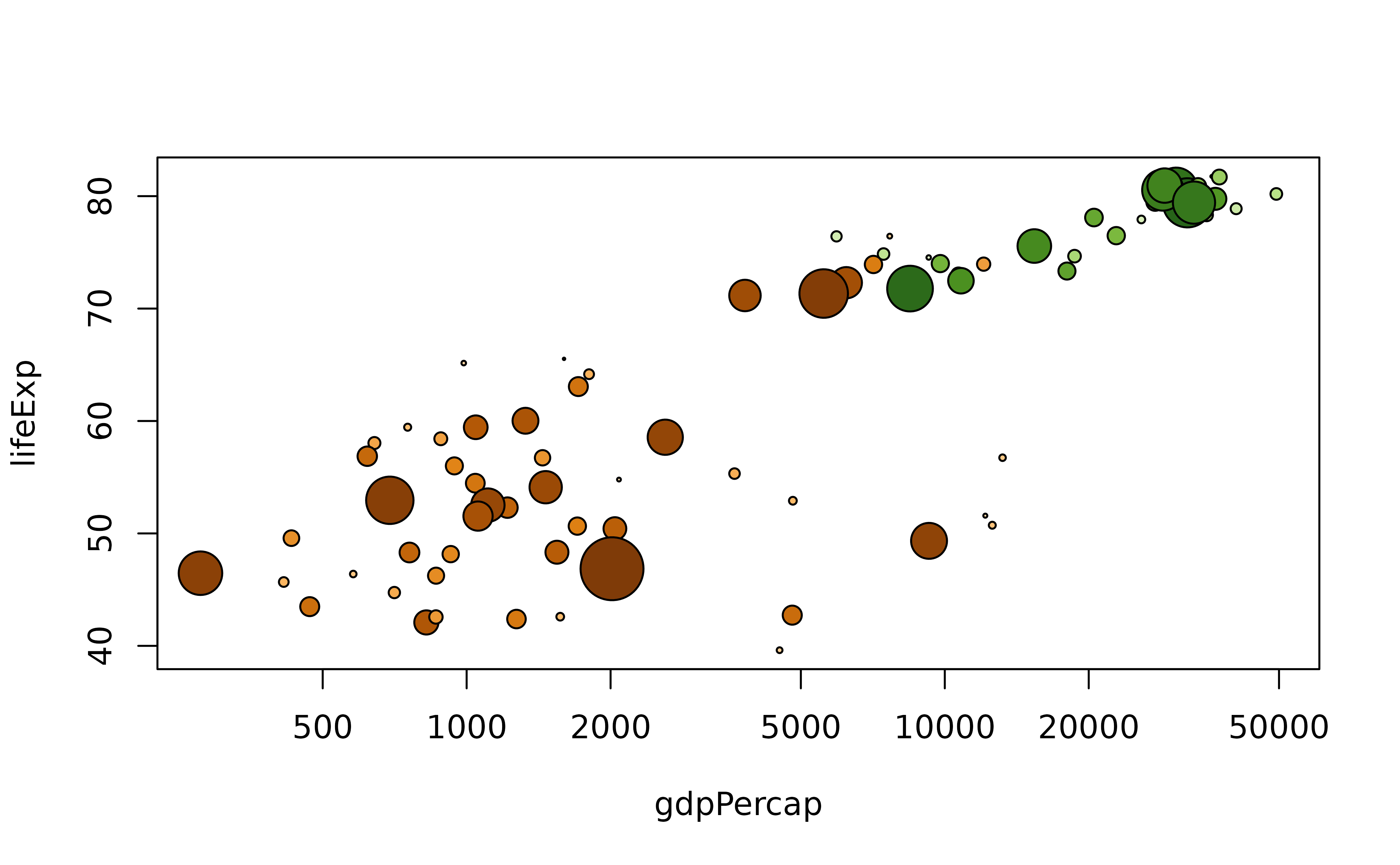
# bubble plot, focus just on Africa and Europe in 2007
keepers <- with(
  gap_with_colors,
  continent %in% c("Africa", "Europe") & year == 2007
)
plot(lifeExp ~ gdpPercap, gap_with_colors,
  subset = keepers, log = "x", pch = 21,
  cex = sqrt(gap_with_colors$pop[keepers] / pi) / 1500,
  bg = gap_with_colors$cc[keepers]
)
ISO 3166-1 country codes
The country_codes data frame provides ISO 3166-1 country
codes for all the countries in the gapminder and
gapminder_unfiltered data frames. This can be used to
practice joining or merging.
library(dplyr)

gapminder %>%
  filter(year == 2007, country %in% c("Kenya", "Peru", "Syria")) %>%
  select(country, continent) %>%
  left_join(country_codes)
#> # A tibble: 3 × 4
#>   country continent iso_alpha iso_num
#>   <chr>   <fct>     <chr>       <int>
#> 1 Kenya   Africa    KEN           404
#> 2 Peru    Americas  PER           604
#> 3 Syria   Asia      SYR           760
What is gapminder good for?
This excerpt has been used in STAT
545, in R-flavored Software
Carpentry Workshops and a ggplot2
tutorial. gapminder is very useful for teaching novices
data wrangling and visualization in R.
Description:
- 1704 observations; fills a size niche between
iris(150 rows) and the likes ofdiamonds(54K rows) - 6 variables
-
countrya factor with 142 levels -
continent, a factor with 5 levels -
year: going from 1952 to 2007 in increments of 5 years -
pop: population -
gdpPercap: GDP per capita -
lifeExp: life expectancy
-
There are 12 rows for each country in gapminder,
i.e. complete data for 1952, 1957, …, 2007.
The two factors provide opportunities to demonstrate factor handling, in aggregation and visualization, for factors with very few and very many levels.
The four quantitative variables are generally quite correlated with
each other and these trends have interesting relationships to
country and continent, so you will find that
simple plots and aggregations tell a reasonable story and are not
completely boring.
Visualization of the temporal trends in life expectancy, by country, is particularly rewarding, since there are several countries with sharp drops due to political upheaval. This then motivates more systematic investigations via data aggregation to proactively identify all countries whose data exhibits certain properties.
How this sausage was made
Data cleaning code cannot be clean. It's a sort of sin eater.
— Stat Fact (@StatFact)
July
25, 2014
The data-raw
directory contains the Excel spreadsheets downloaded from Gapminder in 2008 and 2009 and all
the scripts necessary to create everything in this package, in raw and
“compiled notebook” form.
Plain text delimited files
If you want to practice importing from file, various tab delimited files are included:
-
gapminder.tsv: the same dataset available vialibrary("gapminder"); gapminder -
gapminder-unfiltered.tsv: the larger dataset available vialibrary("gapminder"); gapminder_unfiltered. -
continent-colors.tsvandcountry-colors.tsv: color schemes
In the package’s GitHub repo, these delimited files can be found:
- in the
inst/extdata/sub-directory
Once you’ve installed the gapminder package they can be
found locally and used like so:
gap_tsv <- system.file("extdata", "gapminder.tsv", package = "gapminder")
gap_tsv <- read.delim(gap_tsv)
str(gap_tsv)
#> 'data.frame':    1704 obs. of  6 variables:
#>  $ country  : chr  "Afghanistan" "Afghanistan" "Afghanistan" "Afghanistan" ...
#>  $ continent: chr  "Asia" "Asia" "Asia" "Asia" ...
#>  $ year     : int  1952 1957 1962 1967 1972 1977 1982 1987 1992 1997 ...
#>  $ lifeExp  : num  28.8 30.3 32 34 36.1 ...
#>  $ pop      : int  8425333 9240934 10267083 11537966 13079460 14880372 12881816 13867957 16317921 22227415 ...
#>  $ gdpPercap: num  779 821 853 836 740 ...
gap_tsv %>% # Bhutan did not make the cut because data for only 8 years :(
  filter(country == "Bhutan")
#> [1] country   continent year      lifeExp   pop       gdpPercap
#> <0 rows> (or 0-length row.names)

gap_bigger_tsv <-
  system.file("extdata", "gapminder-unfiltered.tsv", package = "gapminder")
gap_bigger_tsv <- read.delim(gap_bigger_tsv)
str(gap_bigger_tsv)
#> 'data.frame':    3313 obs. of  6 variables:
#>  $ country  : chr  "Afghanistan" "Afghanistan" "Afghanistan" "Afghanistan" ...
#>  $ continent: chr  "Asia" "Asia" "Asia" "Asia" ...
#>  $ year     : int  1952 1957 1962 1967 1972 1977 1982 1987 1992 1997 ...
#>  $ lifeExp  : num  28.8 30.3 32 34 36.1 ...
#>  $ pop      : int  8425333 9240934 10267083 11537966 13079460 14880372 12881816 13867957 16317921 22227415 ...
#>  $ gdpPercap: num  779 821 853 836 740 ...
gap_bigger_tsv %>% # Bhutan IS here though! :)
  filter(country == "Bhutan")
#>   country continent year lifeExp     pop gdpPercap
#> 1  Bhutan      Asia 1972  41.837 1087991  807.6226
#> 2  Bhutan      Asia 1977  44.708 1205659  816.3102
#> 3  Bhutan      Asia 1982  47.872 1333704  946.8130
#> 4  Bhutan      Asia 1987  50.717 1490857 1494.2901
#> 5  Bhutan      Asia 1992  54.471 1673428 1904.1795
#> 6  Bhutan      Asia 1997  58.929 1876236 2561.5077
#> 7  Bhutan      Asia 2002  63.458 2094176 3256.0193
#> 8  Bhutan      Asia 2007  65.625 2327849 4744.6400

read.delim(
  system.file("extdata", "continent-colors.tsv", package = "gapminder")
)
#>   continent n_cty   color
#> 1    Africa    52 #7F3B08
#> 2  Americas    25 #A50026
#> 3      Asia    33 #40004B
#> 4    Europe    30 #276419
#> 5   Oceania     2 #313695

head(
  read.delim(
    system.file("extdata", "country-colors.tsv", package = "gapminder")
  )
)
#>            country   color continent
#> 1          Nigeria #7F3B08    Africa
#> 2            Egypt #833D07    Africa
#> 3         Ethiopia #873F07    Africa
#> 4 Congo, Dem. Rep. #8B4107    Africa
#> 5     South Africa #8F4407    Africa
#> 6            Sudan #934607    Africa
License
Gapminder’s data is released under the Creative Commons Attribution 3.0 Unported license. See their terms of use.
Citation
Run this command to get info on how to cite this package. If you’ve installed gapminder from CRAN, the year will be populated and populated correctly (unlike below).
citation("gapminder")
#> To cite package 'gapminder' in publications use:
#>
#>   Bryan J (2025). _gapminder: Data from Gapminder_. R package version
#>   1.0.1, <https://github.com/jennybc/gapminder>.
#>
#> A BibTeX entry for LaTeX users is
#>
#>   @Manual{,
#>     title = {gapminder: Data from Gapminder},
#>     author = {Jennifer Bryan},
#>     year = {2025},
#>     note = {R package version 1.0.1},
#>     url = {https://github.com/jennybc/gapminder},
#>   }